Posted on
Table of Contents
- Tokenization
- Architecture
- Multi-Head Attention and Transformer Blocks
- Autoregressive Generation
- Pretraining Loop
- Pretraining Results
- Midtraining
- Conclusion
I had been planning to make a YouTube video about this for quite some time. However, just as I was preparing to release it, Andrej Karpathy released an excellent video on the topic, and it quickly went viral. After that, I decided to hold off on recording my version. I am now turning the material into a written guide on the autoregressive transformer architecture. We will implement a GPT-like Large Language Model (LLM) from scratch in Python using PyTorch as the only dependency. I assume familiarity with PyTorch, and for those new to it, Introduction to PyTorch Code Examples from Stanford provides a helpful starting point. Without further ado, let us get started!
The complete code for the GPT-like autoregressive transformer implemented in this article is available here: link. In 222 lines, it automatically downloads the dataset, tokenizes the text, pretrains the model, and generates sample text.
Note that the model implemented and trained in this article, also referred to as the base model, is a sentence completer rather than a chatbot. Converting it into a chatbot involves midtraining, Supervised Fine-Tuning (SFT), and Reinforcement Learning (RL), which are beyond the scope of this article. Still, a pretrained generative LLM is a powerful tool for sampling knowledge.
Tokenization
Given input text, our objective is to generate output text conditioned on that sequence. In traditional transformer models, excluding byte-latent transformers, the initial stage is always tokenization, regardless of whether the architecture is encoder-only (e.g., BERT), encoder-decoder (e.g., T5), or decoder-only (e.g., GPT-2). One straightforward method is character-level tokenization, where each individual character is mapped to a unique token ID. The following zero-dependency Python implementation is designed to handle both encoding and decoding for arbitrary input text data:
import string
class CharacterLevelTokenizer:
"""A character-level tokenizer that treats individual characters as tokens."""
def __init__(self, text: str = string.printable) -> None:
"""Builds the vocabulary from the given text."""
self.vocab: list[str] = sorted(set(text))
self.vocab_size: int = len(self.vocab)
self.char_to_token: dict[str, int] = {char: idx for idx, char in enumerate(self.vocab)}
def encode(self, text: str) -> list[int]:
"""Converts a string into a list of token IDs."""
return [self.char_to_token[char] for char in text]
def decode(self, token_ids: list[int]) -> str:
"""Converts a list of token IDs back into a string."""
return "".join(self.vocab[token_id] for token_id in token_ids)
tokenizer = CharacterLevelTokenizer()
enc = tokenizer.encode("robot") # -> [87, 84, 71, 84, 89]
dec = tokenizer.decode(enc) # -> 'robot'As shown above, CharacterLevelTokenizer treats each individual character as a separate token.
Note that while character-level tokenization is conceptually straightforward, most production systems utilize subword tokenizers to achieve a more optimal balance between vocabulary size and representational capacity. By capturing frequent character sequences as single units, subword algorithms, such as Byte-Pair Encoding (BPE) or WordPiece, significantly enhance computational efficiency compared to more granular methods. However, in this article, we will be using
CharacterLevelTokenizer.
Architecture
At this stage, it may help to look at the transformer architecture as a whole to get a sense of its overall structure. After that, we can break it down and examine each component step by step to see how everything fits together. It may feel a bit overwhelming at first, which is natural, but do not be afraid, since in the end it is simply linear algebra arranged in a certain manner.
from dataclasses import dataclass
import torch
import torch.nn as nn
import torch.nn.functional as F
@dataclass(frozen=True) # We like our dataclasses frozen!
class Config:
"""Transformer config."""
vocab_size: int # Tokenizer vocabulary size
block_size: int # Max sequence length (context window)
n_layer: int # Number of transformer layers
n_head: int # Attention heads per layer
n_embd: int # Embedding dimension (must be divisible by `n_head`)
dropout: float # Dropout probability
bias: bool # Whether `nn.Linear` and `nn.LayerNorm` use bias
@property
def head_size(self) -> int:
"""Returns the per-head dimension (embedding is split evenly across attention heads)."""
return self.n_embd // self.n_head
class Transformer(nn.Module):
"""Autoregressive transformer language model."""
def __init__(self, cfg: Config) -> None:
"""Initializes the building blocks of the transformer."""
super().__init__()
self.block_size = cfg.block_size
self.tok_emb_table = nn.Embedding(cfg.vocab_size, cfg.n_embd)
self.pos_emb_table = nn.Embedding(cfg.block_size, cfg.n_embd)
self.blocks = nn.Sequential(*[Block(cfg) for _ in range(cfg.n_layer)])
self.ln = nn.LayerNorm(cfg.n_embd, bias=cfg.bias)
self.proj = nn.Linear(cfg.n_embd, cfg.vocab_size)
# Weight tying: reduces the total number of parameters without degrading accuracy
# Reference: https://arxiv.org/abs/1608.05859
self.proj.weight = self.tok_emb_table.weight
def forward(self, token_ids: torch.Tensor, targets: torch.Tensor | None = None) -> tuple:
"""Computes logits and optional loss."""
B, T = token_ids.shape
tok_emb = self.tok_emb_table(token_ids)
pos_emb = self.pos_emb_table(torch.arange(T, device=token_ids.device))
emb = tok_emb + pos_emb
out = self.ln(self.blocks(emb))
if targets is None:
logits = self.proj(out[:, [-1], :]) # Last-token projection with time dimension
loss = None
else:
logits = self.proj(out)
loss = F.cross_entropy(logits.view(B * T, -1), targets.view(-1))
return logits, loss
@torch.no_grad()
def generate(
self,
token_ids: torch.Tensor,
max_new_token_ids: int,
temperature: float = 0.7,
top_k: int | None = None,
) -> torch.Tensor:
"""Generates tokens IDs autoregressively."""
self.eval()
for _ in range(max_new_token_ids):
logits, _ = self(token_ids[:, -self.block_size :])
logits = logits[:, -1, :] / temperature
if top_k is not None:
k = min(top_k, logits.size(-1))
threshold = torch.topk(logits, k).values[:, [-1]]
logits[logits < threshold] = -float("inf")
probs = torch.softmax(logits, dim=-1)
next_token = torch.multinomial(probs, num_samples=1)
token_ids = torch.cat((token_ids, next_token), dim=1)
return token_idsLet us focus on the forward method, the core inference function that is also used during generation. After tokenizing the input text, semantic information is captured in tok_emb, which produces token embeddings that represent each token's meaning as a numerical tensor. However, these embeddings do not encode token order. To incorporate positional information, we use learned positional embeddings computed in pos_emb rather than fixed sinusoidal encodings, as learned embeddings are more expressive and can adapt to task-specific positional patterns. The token and positional embeddings are then combined through simple addition to form a unified representation emb that encodes both meaning and position. This additive approach is sufficient, as it breaks permutation symmetry and allows the attention mechanism to infer and model positional structure without requiring more complex operations.
Learned positional embeddings are simple to implement and work well in practice, but they typically tie a model to the maximum sequence length used during training. Many modern architectures instead adopt Rotary Position Embedding (RoPE), which encodes position by rotating query and key vectors with position-dependent angles. This design allows attention to represent relative distances between tokens and often extrapolates more gracefully to longer contexts. For simplicity, however, we will use learned positional embeddings.
Although the line out = self.ln(self.blocks(emb)) appears compact, it encapsulates a substantial portion of the transformer's computational core. Here, self.blocks represents a stack of transformer blocks, each composed of Multi-Head Attention (MHA) mechanisms and Multilayer Perceptrons (MLPs) that progressively refine the token embeddings by modeling complex semantic and contextual relationships across the sequence. Following these deep transformations, self.ln applies layer normalization to stabilize the network and ensure well-behaved gradients. From there, the forward pass branches depending on the objective: during inference (when targets are omitted), the model efficiently isolates the last token's representation before projecting it into vocabulary-sized logits, since predicting the next word only requires this final aggregated context. Conversely, during training, the entire sequence is projected and the resulting logits and targets are flattened to combine the batch and time dimensions, satisfying PyTorch's F.cross_entropy loss requirements.
This cross-entropy calculation represents the core objective of causal pretraining: next-token prediction. By maximizing the likelihood of the correct next tokens over the dataset, the model learns the statistical structure of language. Formally, we minimize the negative log-likelihood of the sequence:
$$\mathcal{L}_{\text{pretrain}}(\theta) = -\sum_{t=1}^T \log P_{\theta}(x_{t} \mid x_{\lt t})$$
Here, \(P_{\theta}\) represents our transformer model parameterized by \(\theta\), and \(x_{t}\) is the target token given all previous context \(x_{\lt t}\).
Multi-Head Attention and Transformer Blocks
While the final projection and loss calculation define the training objective, they are not where the model's main representational power resides. That capability comes from the repeated attention and feed-forward layers inside self.blocks. To understand how the model builds contextual meaning across a sequence, we will next unpack self.blocks(emb) and examine the Block class along with its core components, AttentionHead and MultiHeadAttention, to see how they interact under the hood.
class AttentionHead(nn.Module):
"""A single causal self-attention head."""
def __init__(self, cfg: Config) -> None:
"""Initializes QKV projection and dropout, and cache causal mask to avoid recomputing it."""
super().__init__()
self.qkv = nn.Linear(cfg.n_embd, 3 * cfg.head_size, bias=cfg.bias)
self.dropout = nn.Dropout(cfg.dropout)
self.register_buffer("mask", torch.tril(torch.ones(cfg.block_size, cfg.block_size)))
def forward(self, x: torch.Tensor) -> torch.Tensor:
"""Computes masked single-head self-attention for the input tensor."""
_, T, D = x.shape
q, k, v = self.qkv(x).split(self.qkv.out_features // 3, dim=-1)
attn_scores = q @ k.transpose(-2, -1)
attn_scores = attn_scores * D**-0.5 # Prevent softmax from blowing up
attn_scores = attn_scores.masked_fill(self.mask[:T, :T] == 0, float("-inf")) # Mask future tokens
attn_weights = torch.softmax(attn_scores, dim=-1)
attn_weights = self.dropout(attn_weights)
return attn_weights @ v
class MultiHeadAttention(nn.Module):
"""A Multi-Head Attention (MHA)."""
def __init__(self, cfg: Config) -> None:
"""Initializes multi-head self-attention with output projection and dropout."""
super().__init__()
self.heads = nn.ModuleList([AttentionHead(cfg) for _ in range(cfg.n_head)])
self.proj = nn.Linear(cfg.n_embd, cfg.n_embd)
self.dropout = nn.Dropout(cfg.dropout)
def forward(self, x: torch.Tensor) -> torch.Tensor:
"""Computes masked multi-head self-attention for the input tensor."""
out = torch.cat([head(x) for head in self.heads], dim=-1)
out = self.dropout(self.proj(out))
return out
class Block(nn.Module):
"""Transformer block."""
def __init__(self, cfg: Config) -> None:
"""Initializes a transformer block."""
super().__init__()
self.ln1 = nn.LayerNorm(cfg.n_embd, bias=cfg.bias)
self.mha = MultiHeadAttention(cfg)
self.ln2 = nn.LayerNorm(cfg.n_embd, bias=cfg.bias)
self.mlp = nn.Sequential(
nn.Linear(cfg.n_embd, 2 * cfg.n_embd, bias=cfg.bias), # Flexible: can change to e.g. `4 * cfg.n_embd`
nn.GELU(),
nn.Linear(2 * cfg.n_embd, cfg.n_embd, bias=cfg.bias),
nn.Dropout(cfg.dropout),
)
def forward(self, x: torch.Tensor) -> torch.Tensor:
"""Performs a forward pass: attention + MLP with residuals and layer norms."""
x = x + self.mha(self.ln1(x))
x = x + self.mlp(self.ln2(x))
return xThe AttentionHead class implements a single causal self-attention head. Attention, introduced in the Attention Is All You Need paper, is a directional communication mechanism that allows tokens in a sequence to exchange information, with each token gathering information from others. Each token produces three tensors:
Query: Like asking a librarian a question such as "Which books talk about dinosaurs?" It represents what someone is searching for and is used to scan the catalog to find relevant matches.
Key: Like the labels or table of contents entries in the library catalog. Each key describes what a book or page is about and acts as metadata that helps the query determine which sources are relevant.
Value: Like the actual pages inside the book. After the query matches with the keys, it retrieves the real information or content stored in the values.
The interaction between queries and keys determines how strongly tokens attend to one another, while values carry the aggregated content. In an autoregressive transformer, causal self-attention restricts each token to attend only to previous tokens, preventing future information leakage during training and inference. Furthermore, the queries, keys, and values all originate from the same input sequence. Formally, for the token sequence length \(n\) and input dimension \(d\), query matrix \(Q\), key matrix \(K\), and value matrix \(V\) are projected as \(Q, K, V \in \mathbb{R}^{n \times d}\) and the attention is computed as:
$$\text{Attention}(Q, K, V) = \text{softmax}\big(\frac{Q K^\top}{\sqrt{d}}\big) V$$
where \(QK^\top / \sqrt{d}\) computes scaled similarity scores between queries and keys, with the scaling factor preventing softmax saturation. The softmax converts these scores into attention weights, which in our library analogy represent the relative importance of each page in providing the answer. The weighted sum of \(V\) then produces an output that emphasizes the most relevant information, similar to extracting summarized notes from the most useful pages. In the implementation, attention is computed in the forward method of the AttentionHead class.
In MultiHeadAttention, we implement MHA. Conceptually, MHA consists of several parallel AttentionHead modules whose outputs are concatenated and passed through a final linear projection. This design allows the model to attend to multiple aspects of the input simultaneously, with each head learning distinct relational patterns such as syntactic structure, long-range dependencies, and subtle semantic cues, which enrich the overall representation. We then apply a dropout to the projected output to regularize the MHA module during training. Without this regularization, different heads may co-adapt and learn redundant patterns, and the projection layer after concatenation can become overly confident in certain features. Since transformers have large capacity, this helps reduce the risk of overfitting and encourages the model to learn more diverse and robust representations.
The Block class implements a single transformer block, which serves as a core building unit of the model. The first layer normalization standardizes the input to stabilize training, and the MHA module allows the block to focus on multiple relationships across the sequence, with the residual connection ensuring that the original information is preserved. The second layer normalization prepares the data for the feed-forward network, which expands and transforms each position independently to capture higher-level features, while the GELU activation introduces nonlinearity and the dropout regularizes the output. The second residual connection adds the transformed features back to the input, helping gradients flow more effectively and enabling the block to learn complex patterns without losing essential information. With this, we now understand the line out = self.ln(self.blocks(emb)) and have everything we need to train a GPT-like model.
Autoregressive Generation
During training, the model processes all tokens in parallel using ground-truth targets via teacher forcing. At inference, however, generation is strictly sequential: given an initial prompt of tokens \(x_{1:t-1}\), the model predicts the next token \(x_{t}\), appends it to the sequence, and repeats the process. Specifically, at each step, the model computes unnormalized logits \(\mathbf{z} \in \mathbb{R}^{|\mathcal{V}|}\) across the vocabulary \(\mathcal{V}\) of size \(|\mathcal{V}|\) (vocab_size in our implementation) for the final token position. To balance coherence and variety, these logits are optionally filtered to the top-\(k\) vocabulary subset \(\mathcal{V}_k \subset \mathcal{V}\) and scaled by temperature \(\tau > 0\) for candidate tokens \(v \in \mathcal{V}_k\) (with probability zero for tokens outside this set):
$$P(x_{t} = v \mid x_{\lt t}) = \frac{\exp(z_{v} / \tau)}{\sum_{j \in \mathcal{V}_k} \exp(z_{j} / \tau)}$$
Lower temperatures (\(\tau \to 0\)) sharpen the distribution toward greedy argmax selection, while higher values flatten it, promoting diversity.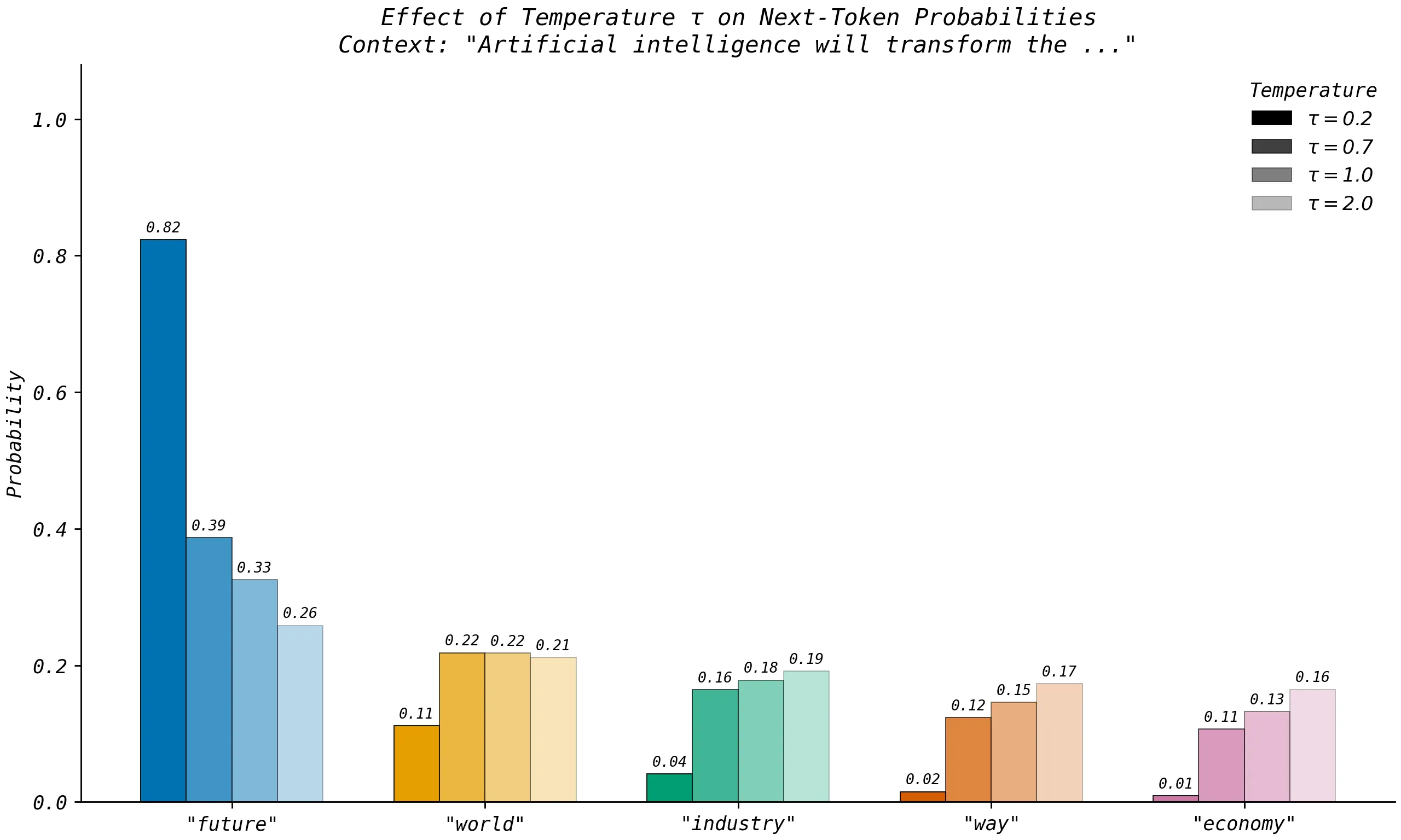
The diagram above demonstrates how temperature modulates sampling dynamics for the prompt "Artificial intelligence will transform the ...". At low temperature (\(\tau = 0.2\)), logit differences are scaled up fivefold, collapsing the distribution so that the top candidate ("future") captures an overwhelming 82% of the probability mass while tail options fall near zero. This produces focused, near-deterministic output suitable for tasks like coding or mathematics, but risks repetitive loops in prose. At moderate temperatures (\(\tau = 0.7\) and \(\tau = 1.0\)), the distribution opens up, granting meaningful likelihood to plausible alternatives like "world" (22%) and "industry" (16%). At high temperature (\(\tau = 2.0\)), logit gaps compress, flattening the probabilities across all candidates and encouraging unexpected completions at the expense of coherence.
Deterministic greedy selection with torch.argmax often produces repetitive loops. Instead, the model samples stochastically using torch.multinomial. This function draws an index from the categorical distribution parameterized by the normalized probabilities:
$$x_{t} \sim \text{Categorical}(P(x_{t} \mid x_{\lt t}))$$
High-probability candidates are chosen most frequently, but lower-probability tokens retain a controlled chance of being selected, enabling natural variation. The sampled token is appended to the context, and to ensure the sequence fits within the context window, the input is cropped to the trailing block_size tokens at each step.
Pretraining Loop
This completes the implementation of the GPT-like transformer! We will now train the model with AdamW and Muon, and generate text.
import urllib.request
def sample_batch(data: torch.Tensor, batch_size: int, block_size: int) -> tuple:
"""Randomly samples training sequences for Next-Token Prediction (NTP)."""
idxs = torch.randint(len(data) - block_size, (batch_size,)) # Random starting positions
token_ids = torch.stack([data[idx : idx + block_size] for idx in idxs]) # Input sequences
targets = torch.stack([data[idx + 1 : idx + block_size + 1] for idx in idxs]) # Same sequences shifted by +1 (NTP)
return token_ids, targets
with urllib.request.urlopen("https://www.gutenberg.org/cache/epub/84/pg84.txt") as f: # Read Frankenstein
text = f.read().decode("utf-8")
tokenizer = CharacterLevelTokenizer(text)
device = torch.device("cuda:0" if torch.cuda.is_available() else "mps" if torch.backends.mps.is_available() else "cpu")
cfg = Config(vocab_size=tokenizer.vocab_size, block_size=32, n_layer=4, n_head=4, n_embd=64, dropout=0.0, bias=False)
max_steps, log_interval, batch_size, learning_rate = 2_000, 10, 256, 1e-3
data = torch.tensor(tokenizer.encode(text), device=device)
model = Transformer(cfg).to(device).train()
n_params, adamw_params, muon_params = 0, [], []
for param in model.parameters():
n_params += param.numel()
(adamw_params if param.ndim < 2 else muon_params).append(param)
print(f"Model parameters: {n_params:,}\n")
adamw = torch.optim.AdamW(adamw_params, lr=3e-4, betas=(0.9, 0.95), eps=1e-8, weight_decay=0.01)
muon = torch.optim.Muon(muon_params, lr=0.02, momentum=0.95, weight_decay=0.1)
for step in range(1, max_steps + 1):
token_ids, targets = sample_batch(data, batch_size, cfg.block_size)
adamw.zero_grad()
muon.zero_grad()
_, loss = model(token_ids, targets)
loss.backward()
adamw.step()
muon.step()
if step % log_interval == 0:
print(f"\rStep {step}/{max_steps} ({step / max_steps:.2%}) | Loss: {loss.item():.4f} ", end="", flush=True)
# Seed the model with the prompt "I am" to kick off text generation
token_ids = torch.tensor(tokenizer.encode("I am"), device=device).reshape(1, -1)
output = model.generate(token_ids, max_new_token_ids=512)[0]
print(f"\n\nOUTPUT:\n\n{tokenizer.decode(output.tolist())}")Pretraining Results
Training logs from under 40 seconds of training on MacBook Pro with Apple M4 Pro chip:
Model parameters: 140,127

Step 2000/2000 (100.00%) | Loss: 1.3831

OUTPUT:

I am the forth which were on his stranger. The light of many our reasun alive in the enter of my
cottagers; there in the murderer, when I walked in
my enemy sat much of spring in its removed. I had not for my friend, and the cottager of the lack of
the wint on the lovely of cestant, and that the old man, but I was entered that
the eviner of my hands. My journey is many beauty will of compassins of the more spully appeared
with meaning a man work was not rease to be macking my own and a
gentle understand even
Midtraining
In production pipelines, base pretraining on web-scale text provides broad world knowledge, but the underlying data distribution is noisy and diluted. As analyzed in a recent survey on mid-training, frontier LLMs bridge this gap through midtraining, also known as continual pretraining. Conceptually, midtraining is a specialized continuation of pretraining that preserves the same autoregressive next-token prediction objective:
$$\mathcal{L}_{\text{midtrain}}(\theta) = -\sum_{t=1}^T \log P_{\theta}(x_{t} \mid x_{\lt t})$$
This stage shifts the focus from broad language understanding toward structured reasoning across three pillars:
Targeted Data Distributions: Upsampling high-utility domains (e.g., code, STEM mathematics, synthetic textbooks, chain-of-thought reasoning, fill-in-the-middle data) while maintaining a replay buffer (typically 10% to 30%) of general pretraining tokens to mitigate catastrophic forgetting.
Learning Rate Annealing: Transitioning into structured cooldown schedules (e.g., warmup-stable-decay, cosine decay) at reduced learning rates. Lower step sizes suppress gradient noise scale variance and help parameters settle into favorable minima.
Context Length Extension: Progressively expanding the sequence length (often from 4K/8K to 32K, 128K, or beyond) via positional encoding adaptations, such as rescaled RoPE frequencies or YaRN, trained on balanced mixtures of long-form and short-form documents. This staged expansion functions as a form of curriculum learning, which has been shown to accelerate the convergence of in-context learning.
Together, these strategies optimize representations and provide a vastly stronger foundation for subsequent training phases.
Conclusion
In this article, we implemented and pretrained a GPT-like autoregressive transformer from scratch using PyTorch, covering character-level tokenization, causal multi-head self-attention, residual connections, next-token prediction with AdamW and Muon, and the foundations of midtraining. While our 140K-parameter model produces only stylistic echoes of Shelley rather than fully coherent prose, the underlying algorithmic blueprint is identical to the one powering frontier systems. At scale, pretraining and midtraining establish broad world knowledge and structured reasoning, yielding capable base models. However, raw base models remain open-ended text completers. Transforming a next-token predictor into a helpful conversational assistant requires post-training, beginning with Supervised Fine-Tuning (SFT), which we explore in Part II.